Goal Programming

Goal programming $GP$ is an extension of Linear Programming $LP$. Essentially GP is LP with multiple objectives. The value of goal programming comes from a need to optimize conflicting objectives which do not have a feasible solution, and where sufficient information to devise an accurate objective function is absent. In both of these cases, goal programming can be used to satisfy objectives as best as possible. Goal programming was first introduced by Dr. Cooper in 1955.

"Mr. Linear Programming": William W. Cooper (1914 - 2012)

Dr. Cooper was a prolific researcher across Operations Research, Management Science, Business, and Accounting. To illustrate his reach: he received four honorary degrees — an M.A. from Harvard University in 1976, and honorary doctorates from The Ohio State University in 1970, Carnegie Mellon in 1982, and the University of Alicante in 1995. With over 500 research articles and 27 books to his name, he was the epitome of an expert in his field.

A map of some of the systems and acronyms in this field.

Brief Overview of Linear Programming

To establish context, consider the foundation of GP: Linear Programming. LP problems seek to optimize a utility function subject to a set of constraints.

Objective function: Defines how the decision variables $\vec{x}$ and cost variables $\vec{c}$ relate to the objective value $Z$.

$$ \text{max } Z = \sum_{j=1}^{n}{\vec{c}_{j} \vec{x}_{j}} $$

Constraints: Provide boundaries for the decision variables. $a_{ij}$ represents the resource requirement for the $i$-th resource and the $j$-th decision variable, and $b_i$ represents the limit for that constraint.

$$ \text{subject to } \quad \sum_{j=1}^{n}{\textbf{a}_{ij} \vec{x}_{j}} \leq b_i \qquad \text{ for } i = 1,\dots,m$$

Variables: Bounds are placed on the variables themselves — for instance, requiring $x_j$ to remain non-negative.

$$ \text{where } \quad \vec{x}_j \geq 0 \quad \text{for } j = 1, \dots, n $$

Example

Problem statement: Maximize profit by choosing how many stools and chairs to produce.

Materials available:
- 75 square feet of wooden sheet (used for chair and stool seats, as well as chair backs).
- 100 wooden rods (used for chair and stool legs).
Materials consumed per product:
- Chair consumes four wooden rods and four square feet of wood.
- Stool consumes three wooden rods and two square feet of wood.
Expected profit from finished goods:
- $50 per chair
- $35 per stool

There are chairs and stools: $n$ = 2. Let $ x_1$ be the number of chairs to build and $ x_2$ the number of stools to build.

There are rods and wooden sheets: $m$ = 2. Let $i = 1$ represent the wooden sheet, and $i = 2$ represent the rods.

$$ \begin{aligned} \text{Maximize} \text{ Profit}\quad & = x_1 \cdot 50 + x_2 \cdot 35 \\ \text{Subject to} \quad & 4 \cdot x_1 + 2 \cdot x_2 \leq 75 \\ & 4 \cdot x_1 + 3 \cdot x_2 \leq 100 \\ \text{Where}\quad & x_1, x_2 \geq 0 \end{aligned} $$

There are three dominant vertices to the 2D solution space, one of which is the optimal solution. Because integer values are required, we can round down each vertex and evaluate profit at each. This yields near-optimal solutions.

Profit at each feasible vertex

All Stools (0, 33) = $1,155
Chairs and Stools (6, 25) = $1,175
All Chairs (18, 0) = $900

For a larger or more critical problem, the branch-and-bound method for integer programming (IP) provides an exact solution. The following Julia implementation demonstrates this:

using JuMP, HiGHS

model = Model(HiGHS.Optimizer)

@variable(model, x1 >= 0, Int)
@variable(model, x2 >= 0, Int)

@constraint(model, 4 * x1 + 2 * x2 <= 75)
@constraint(model, 4 * x1 + 3 * x2 <= 100)

@objective(model, Max, 50 * x1 + 35 * x2)

optimize!(model)

x1_opt = value(x1)
x2_opt = value(x2)
optimal_profit = objective_value(model)

println("Optimal x1: ", x1_opt)             #  x_1    = 4
println("Optimal x2: ", x2_opt)             #  x_2    = 28
println("Optimal profit: ", optimal_profit) #  Profit = $1,180

The exact optimal solution is the nearest feasible integer point to the LP relaxation vertex, which coincides with the intersection of the two active constraints.

Intro to Goal Programming

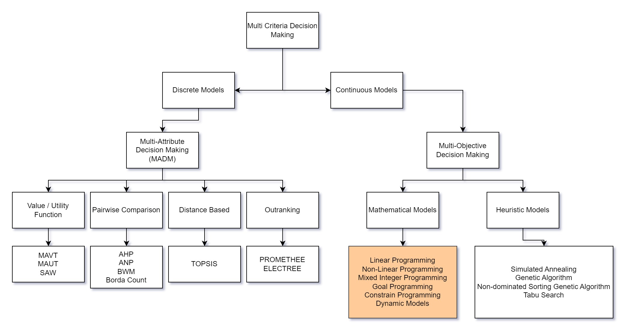
There are two primary methodologies in Goal Programming:

Preemptive (lexicographical): Goals are ranked by priority. A higher-priority goal is treated as infinitely more important than any lower-priority goal. The model is solved top-down, with the highest-ranked goal addressed first.
Non-preemptive (weighted): All objectives are reduced to a common unit and combined into a single system to be solved simultaneously.

This document focuses on the preemptive methodology. Both methods require a decision maker to assign goal priorities, but the preemptive approach makes this hierarchy explicit and avoids the difficulty of finding common units across disparate objectives.

Goal programming is particularly useful when no feasible solution satisfies all goals simultaneously — typically because objectives are in conflict. Both hard constraints and soft goals can coexist in a GP model. The example below illustrates how this combination can produce an infeasible system that goal programming resolves.

Sample Problem

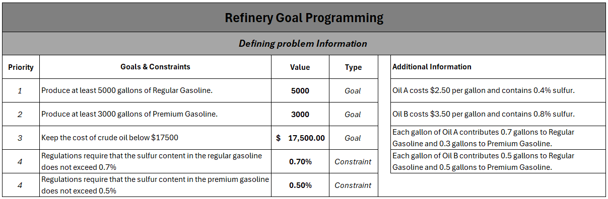
This example is a mixture problem. A refinery blends two types of crude oil — Oil A and Oil B — to produce Regular and Premium Gasoline. The decision makers have established the following ordered priorities:

(Primary): Produce at least 5,000 gallons of Regular Gasoline.
(Secondary): Produce at least 3,000 gallons of Premium Gasoline.
(Tertiary): Keep the cost of crude oil below $17,500.

Additionally, sulfur content must remain below regulatory limits for either product to be sold.

The following information is known:

Oil A costs $2.50 per gallon and contains 0.4% sulfur.
Oil B costs $3.50 per gallon and contains 0.8% sulfur.
Each gallon of Oil A contributes 0.7 gallons to Regular Gasoline and 0.3 gallons to Premium Gasoline.
Each gallon of Oil B contributes 0.5 gallons to Regular Gasoline and 0.5 gallons to Premium Gasoline.
The maximum allowable sulfur content in Regular Gasoline is 0.7%, and in Premium Gasoline is 0.5%.

The goal is to determine which combination of Oil A and Oil B best satisfies the stated objectives. Not all objectives can be fully attained simultaneously. The Desmos visualization below allows you to explore the constraints interactively.

The goal programming formulation is as follows:

$$ \begin{aligned} \text{Maximize} \quad & something & \\ \text{Subject to} \quad & x_1 \cdot 0.7 + x_2 \cdot 0.3 \geq 5000 \\ \quad & x_1 \cdot 0.5 + x_2 \cdot 0.5 \geq 3000 \\ \quad & x_1 \cdot 2.5 + x_2 \cdot 3.5 \leq 17500\\ \quad & x_1 \cdot 0.004 \cdot 0.7 + x_2 \cdot 0.008 \cdot 0.5 \leq (x_1 \cdot 0.7 + x_2 \cdot 0.5) \cdot 0.007\\ \quad & x_1 \cdot 0.004 \cdot 0.3 + x_2 \cdot 0.008 \cdot 0.5 \leq (x_1 \cdot 0.3 + x_2 \cdot 0.5) \cdot 0.005\\ \text{Where}\quad & \vec{x}_1, \vec{x}_2 \geq 0 \end{aligned} $$

Rather than optimizing the objective function directly, we optimize deviations from each goal target. For each goal, the inequality is reformulated as an equality with deviation variables:

$$ \begin{aligned} \text{Minimize } Z = \quad & d_1^{-} + d_2^{-} + d_3^{+}\\ \text{Subject to} \quad & x_1 \cdot 0.7 + x_2 \cdot 0.3 + d_1^{-} - d_1^{+} = 5000 \\ \quad & x_1 \cdot 0.5 + x_2 \cdot 0.5 + d_2^{-} - d_2^{+} = 3000 \\ \quad & x_1 \cdot 2.5 + x_2 \cdot 3.5 + d_3^{-} - d_3^{+} = 17500\\ \quad & -0.0021 \cdot x_1 + 0.0005 \cdot x_2 \leq 0 \\ \quad & -0.0003 \cdot x_1 + 0.0015 \cdot x_2 \leq 0\\ \text{Where}\quad & \vec{x}_1 ,\vec{x}_2 , d_1^{-}, d_1^{+} , d_2^{-}, d_2^{+} , d_3^{-}, d_3^{+} \geq 0 \end{aligned} $$

The deviation variable $d_1^{+}$ captures how much the left-hand side exceeds the right-hand side in the first constraint, while $d_1^{-}$ captures the shortfall. For $\geq$ goals, we minimize $d^{-}$ to drive the solution toward the target. Exceeding a goal carries no additional benefit in this formulation.

Exercise

Download Goal Programming Example

Familiarize yourself with the worksheet.

Figure 1: This section restates the problem.

Figure 2: This section contains the decision variables along with the rates and costs for the problem.

Figure 3: The model output. Goal values and deviations are on the left; constraints are on the right.

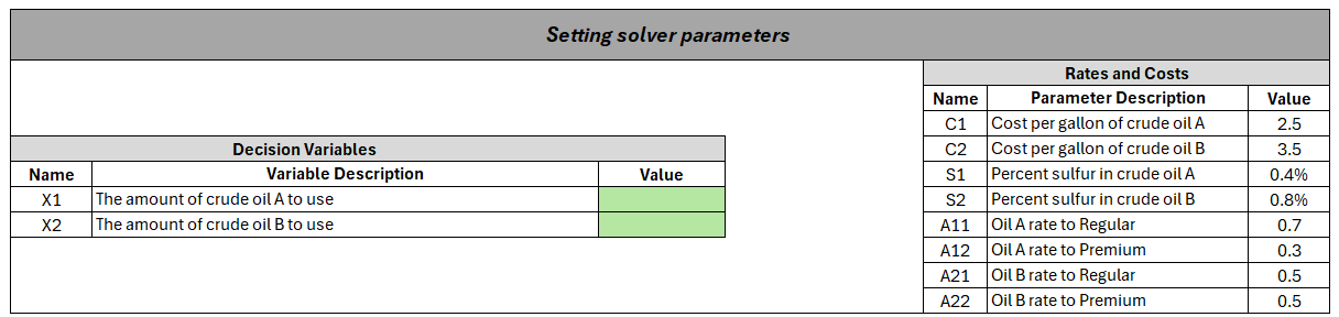
Find values of $x_1$ and $x_2$ that satisfy the constraints and attain as many goals as possible. Use the Excel Solver as follows:

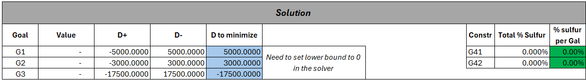
a) First, determine whether Goal 1 (regular gasoline volume) can be met. Minimize the negative deviation, since this is a $\geq$ constraint.

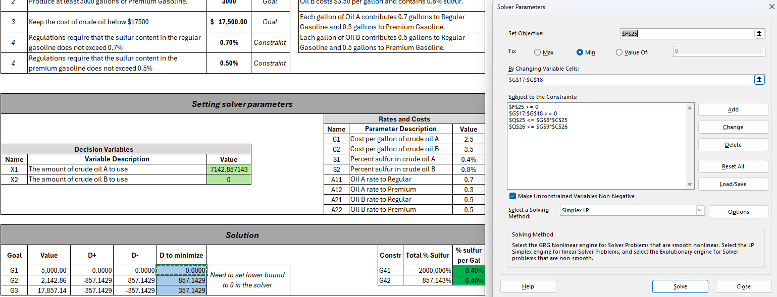Figure 4: Optimize the deviation for Goal 1.

b) Next, determine whether Goal 2 (premium gasoline volume) can be met while holding the deviation for Goal 1 at zero. Minimize the negative deviation, since this is a $\geq$ constraint.

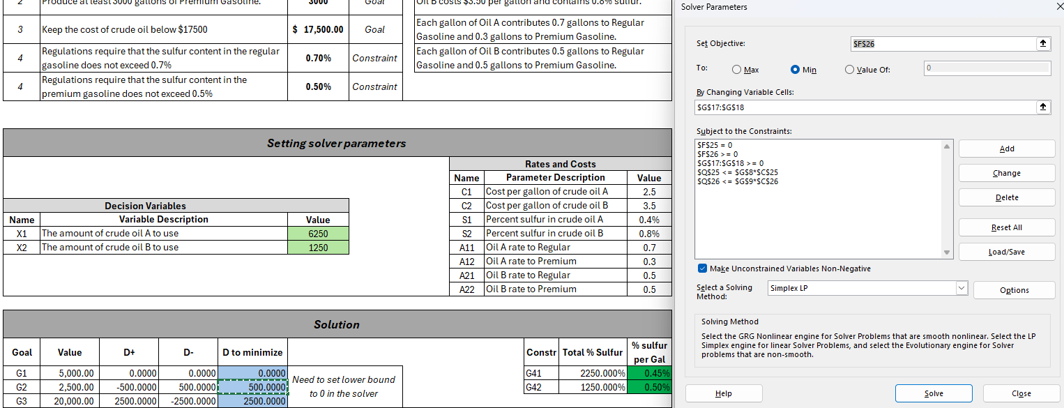Figure 5: Optimize the deviation for Goal 2 while maintaining the solution for Goal 1.

c) Finally, determine whether Goal 3 (crude oil cost) can be met while holding the deviations for Goals 1 and 2 fixed. Minimize the positive deviation, since this is a $\leq$ constraint.

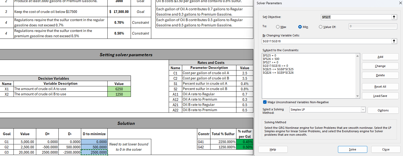Figure 6: Optimize the deviation for Goal 3 while maintaining the solutions for Goals 1 and 2.

The lexicographically optimal solution is to use 6,250 units of Oil A and 1,250 units of Oil B. Goals 2 and 3 are not attained. The sulfur constraint for premium gasoline is binding; the sulfur constraint for regular gasoline has 0.25% slack.

Discussion

What are the strengths of this approach?
What are the limitations of this approach?
Should any goals be revised to make the problem more feasible?
How would changes to the rates or costs of Oil A and Oil B affect the feasibility of the goals?

Bonus Problem

Introduction

An advertising agency is planning a campaign for a client with a budget of $600,000. The client has identified three target audiences and expressed their reach requirements as goals:

Ads should be seen by at least 40 million high-income men (HIM).
Ads should be seen by at least 50 million low-income people (LIP).
Ads should be seen by at least 35 million high-income women (HIW).

Type (per minute)	HIM	LIP	HIW	Cost
Football	7 million	10 million	5 million	$100,000
Soap Opera	3 million	5 million	4 million	$60,000

Formulate the Goals and Constraints

$$ \begin{aligned} \text{Goal } 1 \quad & 7 \cdot x_1 + 3 \cdot x_2 \geq 40 \\ \text{Goal } 2 \quad & 10 \cdot x_1 + 5 \cdot x_2 \geq 60 \\ \text{Goal } 3 \quad & 5 \cdot x_1 + 4 \cdot x_2 \geq 35 \\ \\ \text{Constraint } \quad & 100 \cdot x_1 + 60 \cdot x_2 \leq 600 \\ \\ \text{Where}\quad & x_1, x_2 \geq 0 \end{aligned} $$

Formulate the System with Deviation Variables

$$ \begin{aligned} \text{Minimize} \quad & d_1^{-} + d_2^{-} + d_3^{-} \\ \text{Goal } 1 \quad & 7 \cdot x_1 + 3 \cdot x_2 + d_1^{-} - d_1^{+} = 40 \\ \text{Goal } 2 \quad & 10 \cdot x_1 + 5 \cdot x_2 + d_2^{-} - d_2^{+} = 60 \\ \text{Goal } 3 \quad & 5 \cdot x_1 + 4 \cdot x_2 + d_3^{-} - d_3^{+} = 35 \\ \\ \text{Constraint } \quad & 100 \cdot x_1 + 60 \cdot x_2 \leq 600 \\ \\ \text{Where}\quad & x_1, x_2, d_1^{-}, d_1^{+}, d_2^{-}, d_2^{+}, d_3^{-}, d_3^{+} \geq 0 \end{aligned} $$

LINDO Formulation

MIN d1M + d2M + d3M
ST 
HIM)     7x1 + 3x2 + d1M - D1P               = 40
LIP)    10x1 + 5x2       + d2M - d2P         = 60
HIW)     5x1 + 4x2             + d3M - D3P   = 35

Budget) 100x1 + 60x2 <= 600

Results

Goal 1 is exceeded — positive deviation is acceptable.
Goal 2 is attained exactly — zero deviation.
Goal 3 has negative deviation — the target is not met.